FESTIM 1.4.2 / legacy FEniCS / LAB · RUNS ON ONE CPU
Diffusion across a one-dimensional slab.
Compare concentration and flux with analytical solutions, then measure error on three meshes.
What this model means
Steady diffusion, a hypothetical constant diffusivity and fixed endpoint concentrations. No trapping, decay, surface kinetics or thermal coupling. Deliberately uses the version 1 API with matching dependencies.
J = −D dc/dx; −D d²c/dx² = S
The no-source case gives c = 1 − x and J = 1 in the defined teaching units. The curved case gives c = x(1 − x); its concentration error should fall by about four when the mesh spacing halves.
The run as one scene
The slab of the FESTIM lab, with the steady concentration from the same two cases as the lab on the 32-cell mesh. The model varies in x only; the grid repeats the x profile sideways, which is the model's own symmetry.
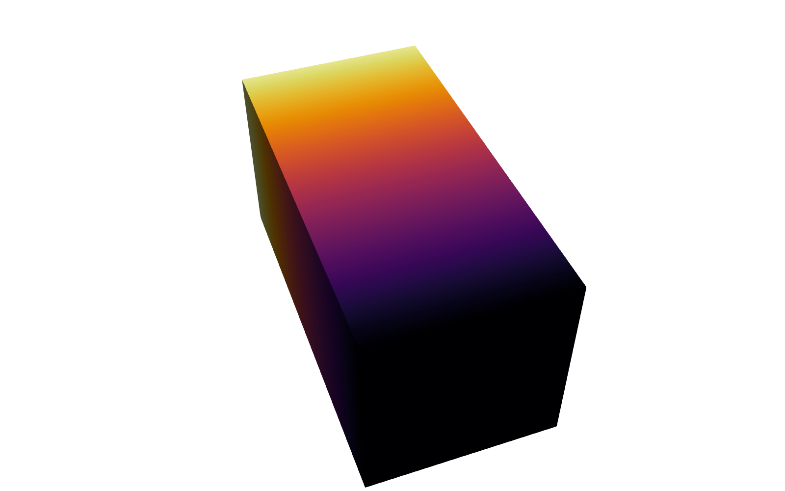
A still from ParaView. Load 3D to turn the scene and pick a field.
Take it with you
Receipt
- Scene run
- FESTIM 1.4.2, Python 3.11.16, Linux-6.8.0-1064-azure-x86_64-with-glibc2.35. 1D steady diffusion; constant D; no trapping, decay or thermal coupling; same as the lab, 32 cells. Addition: XDMF export for ParaView and a 3-D grid that repeats the x profile over y and z. Wall time 18.39 s.
- Geometry
- NVIDIA USD BRep 1.0.0 (exact solids and the display mesh). OpenUSD 0.26.8. Units: L.
- Result layers
- ParaView 6.2, exported headless on the runner.
- Made
- 2026-10-15T11:42:17Z, workflow run 38728950747 ↗.
- Checks against the lab's verified receipt
- L2 error, linear case, scene run vs the lab's verified receipt: 6.837129e-16 vs 6.837129e-16, the same to 1e-12.L2 error, curved case, scene run vs the lab's verified receipt: 0.0001782951 vs 0.0001782951, the same to 1e-12.
- Script hashes
- scene run
1ecaf4e9b61e790c…; the lab's scriptbaf8a95d4ee68db1…(unchanged).
Rules this scene keeps
- Geometry is for display, never solver input. The solver used its own one-dimensional mesh.
- Each concentration field comes from a real FESTIM 1.4.2 run of the same case as the lab. Its receipt is in this scene.
- Units are the lab's hypothetical units: L = 1, D = 1, concentration scale 1.
- Nothing here predicts a real fusion component.
Run the lab
You need
- A computer with Linux x86-64, Windows with WSL2 Ubuntu, or a Mac (Apple silicon, native). Native Windows is not tested.
- Conda. Conda installation guide ↗. On Windows, install WSL2 Ubuntu ↗ first, then install Conda inside Ubuntu.
- An internet connection. Installation takes 5 to 15 minutes. The run itself takes about 15 seconds.
Words used below. A terminal is the window where you type commands. An environment is a separate set of programs installed only for this lab. The receipt is the file results/receipt.json that the lab writes when it finishes.
1. Download and extract the lab
Download FESTIM 1.4.2 / legacy FEniCS lab (.zip) ↓Extract the ZIP in your Linux home folder. On Windows, the folder must be inside Ubuntu, not on the Windows desktop.
Open a terminal in the extracted folder. Read README.md before you change anything.
2. Create the environment
Type the first command for your computer. Press Enter. Wait until the prompt returns. This takes 5 to 15 minutes.
conda create -n vtb-festim --file explicit-linux-64.txtconda create -n vtb-festim --file explicit-osx-arm64.txtType the second command. Press Enter. The prompt now starts with
(vtb-festim).conda activate vtb-festim3. Run the lab
Before you run: write down the answer you expect from the equation above.
Type the command below. Press Enter.
OMP_NUM_THREADS=1 OPENBLAS_NUM_THREADS=1 python run.pyRead the last line in the terminal. It must contain
VTB_RECEIPTandstatus: passed.If it does not: stop. Copy the error message. Compare your installed packages (
conda list) with the explicit file you used. Do not change the seed.4. Read the receipt and keep it
Open
results/receipt.json. Compare the numbers with the equation above.Open the concentration and flux tables. Compare 8, 16 and 32 cells. The linear case matches exactly; the curved case shows the mesh error, which falls by about four each time the cell size halves.
Keep the receipt, the lock file and any change you made together. A new run replaces the files in
results/, so copy the folder first if you want to keep an earlier run.5. Change one thing
Open
run.pyin a text editor. Change one number: the source S or the number of cells. Predict the effect first. Then run the command from step 3 again.The new receipt shows a different script hash. That is correct. It means the run is yours, not the packaged example. Write down what you changed and what you predicted.
YOUR ACCOUNT · NO INSTALL
Run this lab here
A Linux runner runs the packaged script with the numbers you choose and sends the receipt to your account. You can change only S (volumetric source in the curved case) and N (cells in the mesh), each inside a fixed range. Predict the result first, as in step 5. The receipt is labelled “Hosted”, never “Unchanged example”.
YOUR ACCOUNT
Add this run
Keep the run in your account. Do this after step 4, and again after each change in step 5.
Verification and provenance
Verified with the real solver on Linux x86-64 (Ubuntu 22.04 CI). Run time: 12.85 seconds. Peak memory: 268.0 MiB. These numbers include program start-up and exclude installation. Your computer will differ.
Also verified on macOS 14 arm64 (GitHub macos-14 CI), run 37693541442: the same script passed every check in 12.61 seconds. The Mac lock explicit-osx-arm64.txt and its receipt are in the download.
Native Windows is not tested for this lab. Each download includes the original teaching code, the MIT license, dependency license links, the analytical checks, and the verification receipts. The solver packages keep their own licenses.
Follow the reproducibility journey →